Module 15: Data Science with Polars

Lecture 33: Wednesday, April 22, 2026, and
Lecture 34: Friday, April 24, 2026.
Code examples

The Polars Library

Polars is a dataframe library written in Rust.

Dataframes: If you’ve used pandas, the concept of a dataframe should be familiar to you: A Dataframe is a two dimensional heterogeneous tabular data structure. It consists of labeled columns and rows which may hold data items of different types. In many ways, it is akin to a spreadsheet that you can programmatically interact with in your desired language to perform data analysis.

Polars is implemented in Rust for high performance. We will see a couple of cool features it supports below. You can use Polars in Rust, but you can also use it in Python, as the Polars developers have created a Python embedding for it (even though all of its internals are implemented in Rust behind the scenes).

Compared to pandas, Polars provides additional features:

1. It automatically optimizes queries before executing them (more on this below).
2. It automatically runs components of the queries (i.e., sub-queries) in parallel.

Application Scenario

We will start with an application scenario. Say we have the following csv data stored in a csv file called albums.csv.

band,album,rating
Humanity's Last Breath,Humanity's Last Breath,7
Meshuggah,Nothing,5
Humanity's Last Breath,Ashen,5
Meshuggah,Nothing,4
Vildhjarta,Masstaden,4
Humanity's Last Breath,Ashen,4
Vildhjarta,Dar Skogen Sjunger,4
...

Each line in this csv file represents a row of data consists of the rating that one user has provided for a given album. For example, the first data line above represents a user rating Humanity’s Last Breath self-titled debut album with a 7 out of 5 (yes, it’s that good). The data above contains a handful of lines for demonstration reasons. Assume that the actual data set contains many, perhaps millions, of ratings.

Our goal is to use Polars to analyze this data, and in particular, compute the average rating for some albums of interest.

Abstractly, you can view our query as consisting of these logical steps:

GROUP BY [band, album]
COMPUTE average(rating) per group
FILTER BY album = '<desired album>'

You will see a better language for describing queries like this called SQL in DS 310. But for now, all we need is to understand this query intuitively at a high level.

We are going to see two ways we can perform this query in Polars, the first is using eager execution, the second using lazy execution.

We provide the complete code for these examples in our repo along with instructions for how to generate an albums dataset and how to run the code. As you go through the notes below, make sure you also follow in the provided sample code and to run and experiment with the code one part at a time.

Eager Data Analytics with Polars

Eager execution is the “normal” kind of execution where when we write down some piece of code or expression, the computer executes that expression directly (also called eagerly) as soon as it encounters it. For example, if the computer gets to a line that says let x: i32 = y + 10; while executing a Rust program, it reads the value inside of y, adds 10 to it, and puts the actual and complete result in a new variable called x.

Let’s think how we could express the query above normally (using Polars’ eager API).

Step 0: Import Polars.

We begin by adding Polars as a dependency in our Cargo.toml file.

polars = { version = "0.53.0", features = ["polars-io", ...] }

We must also import the different types and functions we want to use from Polars.

use polars::prelude::{CsvReadOptions, CsvReader, DataFrame};
// or use polars::prelude::*; to import everything

Step 1: Read data from the CSV file.

Polars provides a CsvReader type that can read .csv files and transform them into Dataframes stored in the program’s memory. To use the CsvReader, we must first configure it. Polars provides a lot of configurations that you can use, but in our case, all we need is to let the reader know that the file contains a header row in the beginning and where the file is located.

let reader: CsvReader<File> = CsvReadOptions::default()
    .with_has_header(true)
    .try_into_reader_with_file_path(Some("albums.csv".into()))
    // functions that start with try_ usually return a Result<T, Error>
    // we unwrap that Result below to get the CsvReader we are looking for.
    .unwrap();

Now that we have a reader ready, we can ask it to read the entirety of the file in one go.

let data: DataFrame = reader.finish().unwrap();

Now that we have data of type DataFrame, we can use any of its methods as we like, e.g., to explore what the data looks like:

println!("{}", data);
println!("Number of rows in dataset {}", data.height());
println!("First row in dataset {:?}", data.get_row(0).unwrap());

Which gives us an album similar to the below:

shape: (7, 3)
┌────────────────────────┬────────────────────────┬────────┐
│ band                   ┆ album                  ┆ rating │
│ ---                    ┆ ---                    ┆ ---    │
│ str                    ┆ str                    ┆ i64    │
╞════════════════════════╪════════════════════════╪════════╡
│ Humanity's Last Breath ┆ Humanity's Last Breath ┆ 7      │
│ Meshuggah              ┆ Nothing                ┆ 5      │
│ Humanity's Last Breath ┆ Ashen                  ┆ 5      │
│ Meshuggah              ┆ Nothing                ┆ 4      │
│ Vildhjarta             ┆ Masstaden              ┆ 4      │
│ Humanity's Last Breath ┆ Ashen                  ┆ 4      │
│ Vildhjarta             ┆ Dar Skogen Sjunger     ┆ 4      │
└────────────────────────┴────────────────────────┴────────┘
Number of rows in dataset 7
First row in dataset Row([String("Humanity's Last Breath"), String("Humanity's Last Breath"), Int64(7)])

Step 2: Group by band and album.

Before we can compute the average, we must tell Polars how we want to group the records we want to average first. E.g., if we just ask to average without any grouping, we will get one number: the average of all the ratings across all albums and bands.

Here, we want to group by the band and album.

let groups: GroupBy =
    data.group_by(["band", "album"]).unwrap();

Notice that the result of this operation is something of type GroupBy. This represents a collection of many DataFrames, one per group.

Step 3: Compute the average within each group.

In Polars, the API for computing the average is called mean().

let averages: DataFrame = 
    groups.select(["rating"]).mean().unwrap();

Note that:

1. We asked to compute the mean from the groups, not from the original data.
2. The result is a DataFrame where each row represents one group (i.e. one band and album) along with the average for that group.

Step 4: Filter the averages to only keep the album of interest.

Let us say we want the average rating for the album Ashen.

// Get the album column, and ensure that it contains strings.
let albums = averages.column("album").unwrap().str().unwrap();
let condition = albums.equal("Ashen");
let result: DataFrame = averages.filter(&condition).unwrap();

Note that the result here is again a DataFrame. This is a recurring pattern: Polars provides APIs that allows you to manipulate a DataFrame to create a new derived DataFrame, e.g., by filtering or aggregating the data (among many other available operations).

Now, we can print this final result:

println!("{}", result);

shape: (1, 3)
┌────────────────────────┬───────┬─────────────┐
│ band                   ┆ album ┆ rating_mean │
│ ---                    ┆ ---   ┆ ---         │
│ str                    ┆ str   ┆ f64         │
╞════════════════════════╪═══════╪═════════════╡
│ Humanity's Last Breath ┆ Ashen ┆ 4.5         │
└────────────────────────┴───────┴─────────────┘

Success!

You can view the full code in the provided eager.rs.

Now, follow the instructions in the README in the accompanying code on our repo and generate a much larger file, e.g., with 50 million rows, and then execute the above code against it.

cd module_15_polars
# Generate a large dataset with 50 million rows
python3 albums.py 50000000 > albums50M.csv
# Analyze the dataset using the eager version of our code
cargo run --bin eager -- albums50M.csv

On my computer, this took around 6 seconds to complete. It also used a lot of memory. Follow the instructions in the README to look at the memory consumption, specifically the peak memory consumption (sometimes called maximum resident set size), which is the maximum amount of memory that was used at any point during execution.

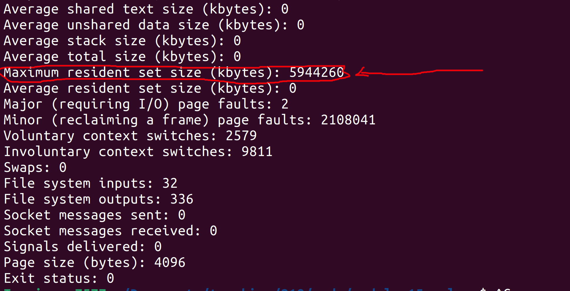
On my computer, you can see that the peak memory consumption was 5944260 Kilobytes (roughly 5.9 Gigabytes). The input albums50M.csv file is roughly 1.4 Gigabytes, so this peak memory consumption makes some sense since we read the entire file to memory in one shot, then operate over it (which inadvertently creates some copies of it behind the scenes).

Note: depending on your OS, the output may be differently formatted (e.g. in bytes instead of kilobytes on mac), and the maximum resident set size might be called something else (e.g., peak memory consumption on mac). Note: if your computer has a small RAM, it might start lagging when working with the full 50 million entries dataset. In that case, feel free to generate and use a smaller dataset (e.g., 10 or 5 millions).

Can we do better? Let’s find out next.

Manually Optimizing Eager Queries

Let’s review the query we have written above and think about whether we can (manually) optimize it to reduce its runtime and memory usage!

READ (entire) CSV file
  -> GROUP BY [band, album]
  -> COMPUTE average(rating) per group
  -> FILTER BY album == "Ashen"
  -> PRINT ALL

Detour: Query Plan

The above summary of the query is often called a plan. There are many flavors of plans out there, from high level logical plans (similar to what we wrote above) to much lower level plans that, e.g., show nearly the full details of every operation that gets performed.

Note for the final exam: You will be asked to write and manipulate query plans on the exam, so familiarize yourself with them. You can use the exercises at the end of these notes to practice. The exact syntax you use is not important, as long as you show us the right steps in the right order.

End of Detour: Back to (Manually) Optimizing the Query

Is there something we can do to this plan (and the underlying query) to optimize it?

The key observation is finding out whether the query as planned performs any useless computation, e.g., if earlier parts of the query computes some data that later parts of the query disregard!

In this case, our query begins by computing the average rating for every group of band and album. That’s a lot of work, both for grouping and for computing the average.

But, notice that later on, the query filters out all of these groups (and their averages) except for one album "Ashen". This means that all the work done previously to group and compute averages for other albums was wasted/meaningless work.

We shouldn’t be asking the computer to do meaningless work! So, what can we do to avoid that? Ideally, we will only ask the computer to group and aggregate ratings for the specific album we want. It turns out that we can do that by rewriting (in this case, re-ordering) the query.

READ (entire) CSV file
  -> FILTER BY album == "Ashen"
  -> GROUP BY [band, album]
  -> COMPUTE average(rating) per group
  -> PRINT ALL

This new plan performs the filter first, which allows us to remove the vast majority of the dataset. Then, we perform the group by and average on only the remaining data.

We can go even further: since we know all the data that remains after the filter corresponds to the album "Ashen", we do not need to group by album anymore!

READ (entire) CSV file
  -> FILTER BY album == "Ashen"
  -> GROUP BY [band]
  -> COMPUTE average(rating) per group
  -> PRINT ALL

This seems easy enough to do with the plan, but how do we tell Rust and Polars that we want this version of the query instead of the one we wrote in the previous section!? Well, we have to rewrite our Rust code to reflect this new plan.

let data: DataFrame = /* read csv file using CsvReader */;

// Filter by album == Ashen.
let albums = data.column("album").unwrap().str().unwrap();
let condition = albums.equal("Ashen");
let filtered_data: DataFrame = data.filter(&condition).unwrap();

// Group by the band then compute the average rating per group.
let groups = filtered_data.group_by(["band"]).unwrap();
let result = groups.select(["rating"]).mean().unwrap();

You can find the full modified code in the provided eager_optimized.rs.

Follow the instructions to run the optimized query and observe its run time and memory usage.

On my computer, when I ran the optimized code on the albums50M.csv dataset, the runtime went down to around 3.5 seconds. Furthermore, the peak memory consumption went down to around 3.8 Gigabytes! Big improvement!

Manual Optimizations Gone Wrong

Manually optimizing this query seemed easy enough, but that’s because this particular query is pretty simple. In generally, manual optimizations of this kind can be very risky if the programmer is not experienced and is not thinking carefully about what they are doing.

There are two ways manual optimizations can go wrong:

1. The programmer misses some additional opportunity for optimizations and ends up with a program with subpar performance.
2. The programmer rewrites their query or code in a way that actually changes what the query computer (rather than simply how it computes it) and end up with wrong results.

There errors may occur either during the logical optimization (i.e., when the programmer is rearranging the plan) or when they are changing their code to reflect the new optimized plan (e.g., by adding some unintentional bug to the code).

Consider the last plan above. The plan performs a group by band and then computes the average. But, is that really needed? Why not do this instead:

READ (entire) CSV file
  -> FILTER BY album == "Ashen"
  -> COMPUTE average(rating)
  -> PRINT ALL

Consider these two scenarios:

1. The query begins by filtering data for any album not named "Ashen". This is a very peculiar album name, and it is likely that Humanity's Last Breath is the only band that has released an album with that name. In this case, it would be OK to get rid of the group by and simply compute the average directly! So, in this case, the optimized plan we came up with could be optimized even further.
2. Imagine we were looking for (and thus filtered by) some other album whose name is less peculiar. For example, the great King Crimson released a terrific album called Red in 1974. However, Taylor Swift also released a much worse album named Red as well in 2012. If we remove the group by and directly compute the average, we would mix the great ratings the King Crimson got with the mediocre Taylor Swift album, resulting in a meaningless average rating. In this case, we would have incorrectly optimized the query and caused it to produce incorrect outputs.

The conclusion: optimizing queries and programs is dangerous business! You need to take into consideration a variety of constraints, including ones that are not explicitly expressed in the code and are instead related to contextual information you may know about the data and the business logic.

Fear not though! The next section will describe a way to have Polars automatically optimize the queries for you!

Automatically Optimized Data Analytics Query Using Lazy Execution

Let’s revisit our hand optimized query plan from above:

READ (entire) CSV file
  -> FILTER BY album == "Ashen"
  -> GROUP BY [band]
  -> COMPUTE average(rating) per group
  -> PRINT ALL

Motivation

As discussed, this is a correct query plan, but one that is prone to errors if the programmer decides to attempt to optimize it further (by removing the group by).

At the same time, this query misses another important optimization: the query reads the entirety of the CSV file to memory, then it filters out the irrelevant data.

This means that prior to the filter, the entire dataset sits in memory! Only after all of it has been read does the program start filtering out irrelevant data.

This is a serious problem: imagine if the data was so big that it would not even fit in RAM (e.g., 100GB). This is not an unrealistic scale for many datasets out there. Even in such a case, the relevant data (i.e., ratings for the album “Ashen”) may constitute only a small portion of this data set that does fit in memory (e.g., 100MB).

Thus, a much better approach is to filter the data as we read it from the file, e.g., one row at a time. This means the program will only ever store relevant data in memory, reducing the peak memory usage. Ofcourse, even in this case, the program would still need to go through the entire dataset file in order to find the relevant data, but it can do so while using less memory.

How can we implement something like this? Well, we can implement our one CSVReader that:

1. In a for loop, reads one line at a time from the file.
2. For each line, it applies the filter, and pushes the row of data to the DataFrame if meets the filter.

This is doable, but would require writing a bunch of code to read files one line at a time, parse comma-separate rows, etc. Furthermore, it would have to deal with a bunch of edge cases, e.g., what if one row spans several lines?

Polars LazyReader

Fortunately, Polars provides us with a reader that can do that for us so we do not have to worry about it. This is called a LazyReader.

We can use a LazyReader as follows:

let data: LazyFrame = LazyCsvReader::new("albums.csv".into())
        .with_has_header(true)
        .finish()
        .unwrap();

Compared to the previous Polars code we saw in the previous two sections, we have two big differences here:

1. We are using LazyCsvReader instead of CsvReader.
2. With CsvReader, the .finish().unwrap() code used to read the entire file and return a DataFrame. However, with LazyCsvReader, that code returns LazyFrame instead.

LazyFrame

So, what are the differences between DataFrame and LazyFrame? Well, both of them represent heterogeneous tabular data. However, while DataFrame has the entirety of the dataset within its content and in memory, LazyFrame is merely a placeholder: it does not actually have any data yet! It is merely an object that Polars gives us that allows us to describe the query we want, without reading any data or executing that query yet.

How do I know this? Well, for one, the Polars documentation says so. But also, if we try to print the LazyFrame or even get the count of rows in it, we will get some compile errors from Rust telling us those APIs are not available for it!

let data: LazyFrame = /* lazy read from file */;
println!("{}", data);
println!("Number of rows in dataset {}", data.height());
println!("First row in dataset {:?}", data.get_row(0).unwrap());

error[E0277]: `LazyFrame` doesn't implement `std::fmt::Display`
   |
   |     println!("{}", data);
   |               --   ^^^^ `LazyFrame` cannot be formatted with the default formatter
  
error[E0599]: no method named `height` found for struct `LazyFrame` in the current scope
     |
     |     println!("Number of rows in dataset {}", data.height());
     |                                                   ^^^^^^

error[E0599]: no method named `get_row` found for struct `LazyFrame` in the current scope
   |
19 |     println!("First row in dataset {:?}", data.get_row(0).unwrap());
   |                                                ^^^^^^^ method not found in `LazyFrame`

If the LazyFrame does not have any data in it, then what’s its use!? Well, we can still use the functions and APIs that Polars provides to express what query we want to execute using the LazyFrame. The query would not get executed just yet, since LazyFrame is merely a placeholder, but now Polars would know what our desired query is. When we have expressed the entire query, we could then ask Polars to optimize it and execute it as it sees fit!

For example, we can state the query in the same shape we started the first section with:

let data: LazyFrame = /* lazy read from file */;

let output: LazyFrame = data
  .group_by([col("band"), col("album")])  // returns a LazyGroupBy
  .agg([col("rating").mean()])            // returns a LazyFrame
  .filter(col("album").eq(lit("Ashen")));

Compared to the eager version of the query, the main differences are:

1. The code is shorter and less verbose, this is because Polars spent more time carefully improving their Lazy API, since it is their recommended way of using Polars.
2. The output variable has type LazyFrame: no computation over data has been executed yet!

Automatic Plan Rewriting

We can ask Polars to show us the plan it has for the query we just wrote.

#![allow(unused)]
fn main() {
println!("Initial Plan: {}", output.explain(false).unwrap());
println!("Optimized Plan: {}", output.explain(true).unwrap());
}

This shows us the following output:

Initial Plan: FILTER [(col("album")) == ("Ashen")]
FROM
  AGGREGATE[maintain_order: false]
    [col("rating").mean()] BY [col("band"), col("album")]
    FROM
    Csv SCAN [albums50M.csv]
    PROJECT */3 COLUMNS
    ESTIMATED ROWS: 43922804
    

Optimized Plan: AGGREGATE[maintain_order: false]
  [col("rating").mean()] BY [col("band"), col("album")]
  FROM
  Csv SCAN [albums50M.csv]
  PROJECT 3/3 COLUMNS
  SELECTION: [(col("album")) == ("Ashen")]
  ESTIMATED ROWS: 43922804

Note that Polars outputs the plan in a slightly different format than ours from earlier. You should read Polars plans from the bottom up, instead of the other way around. This is a common way of representing plans that you may encounter in other contexts as well (e.g. database queries).

However, the plan still more or less shows the same information as our previous plans. Look at the initial plan. This encodes the query as we wrote it:

1. It reads the Csv file (Csv SCAN), which also includes a projection (PROJECT */3 columns). This indicates that the query wants to project (or keep) all 3 columns in the dataset.
2. It groups by the band and album and aggregates by computing the average rating for each group.
3. It filters based on album == "Ashen".

On the other hand, the optimized plan looks different, and is in fact a bit more akin to our hand optimized plan:

1. It reads the Csv file (Csv SCAN) while also performing the filter by album == "Ashen" during the read (so only relevant data is read into memory).
2. It groups by band and album and computes the average rating per group.

Finally: Executing the Query and Getting the Output

When we are happy with the query and have expressed all of its components, we can ask Polars to go ahead and actually run this query now.

It is only at this point that Polars reads any data from the file and runs the components of the query. Polars does this in one go: it will return to us the final output of the query, but will not show us any intermediate results. This gives Polars the freedom to rewrite the query and plan as it sees fit.

// Ask polars to run the query (with optimizations).
let result: DataFrame = output.collect().unwrap();
println!("{}", result);

Note that the type of result is DataFrame, since calling .collect() instructs Polars to stop being lazy and actually read the data and execute the query! Now, we can do whatever we want to the result and its data, including printing it, or using it for future eager queries, etc.

You can find the complete lazy code in the provided lazy.rs.

Follow the instructions in the README to run this code. On my computer, this code takes roughly the same amount of time as the hand optimized query (around 3.5 seconds), but it has much lower peak memory usage at under 2GB!

Note on Automatic Optimization

Polars performs query optimizations based on query rewriting rules.

These are hand written rules that the Polars developers designed. They prioritize safety and correctness: they are meant to be correct transformations that would not change the output of any possible query and are guaranteed to never be incorrect.

As a result, these rules may miss some available optimizations that are based on business logic or contextual information about the data that are known to us, e.g., from lived experience or fuzzy specification, but not known to Polars in the data schema or the query information.

This is a common theme in many other cases as well, including how SQL databases automatically optimize queries.

In practice, achieving the best performance is a cooperative and iterative task where the query developers use the automatic optimized plans as a starting point, and then may do some further rewriting or introduce additional information (e.g., indices, schema information) and ask the system to re-optimize the plan again. Query developers may do this over several iterations, including benchmarking different versions of the query, until they are satisfied with their optimizations.

Exercises

Exercise 1

We are using the same albums data set as above. You are given the following logical query plan.

READ (entire) CSV file
  -> GROUP BY [band, album]
  -> COMPUTE max(rating) per group
  -> FILTER BY band == "Meshuggah"
  -> PRINT ALL

Question 1: Describe what this query does in English.

Question 2: You are tasked with optimizing this query by rewriting or reordering the plan. Provide the best optimized plan you can come up with that is also correct (i.e., do not change the output of the query).

READ CSV file AND FILTER BY band == "Meshuggah"
  -> GROUP BY [album]
  -> COMPUTE max(rating) per group
  -> PRINT ALL

Exercise 2

We are using the same albums data set as above. You are given the following logical query plan.

READ (entire) CSV file
  -> GROUP BY [band]
  -> COMPUTE distinct count(album) and average(rating) per group
  -> SORT BY average(rating) DESCENDING ORDER
  -> FILTER BY distinct count(album) >= 2
  -> PRINT FIRST ROW

Question 1: Describe what this query does in English.

Question 2: You are tasked with optimizing this query by rewriting or reordering the plan. Provide the best optimized plan you can come up with that is also correct (i.e., do not change the output of the query).

READ (entire) CSV file
  -> GROUP BY [band]
  -> COMPUTE distinct count(album) per group
  -> FILTER BY distinct count(album) >= 2
  -> COMPUTE average(rating) per group
  -> SELECT ROW WITH max(average(rating))
  -> PRINT ALL

Exercise 3

You are given a dataset with all of BU’s student records across its history. The data set includes one row per student and has the following columns: name, BUID, email, department, degree, GPA, graduation year.

You are also given the following logical query plan:

READ (entire) CSV file
  -> GROUP BY [department]
  -> FILTER BY GPA > 3.5
  -> COMPUTE count per group
  -> PROJECT [department, count]
  -> PRINT ALL

Question 1: Describe what this query does in English.

Question 2: You are told that this query is important for the registrar office. Specifically, the registrar office is looking for the count of distinct students who graduates with a GPA higher than 3.5.

In other words, if a student graduated twice, i.e. once with a bachelor’s and then once again later with a master’s, they should count only once!

In light of this new information, you notice a bug with previous query: it counted such students twice! So you set out to fix this bug and produce this new query plan:

READ (entire) CSV file
  -> GROUP BY [department]
  -> FILTER BY GPA > 3.5
  -> COMPUTE distinct count(name) per group
  -> PROJECT [department, distinct count(name)]
  -> PRINT ALL

Does this query compute the desired information correctly? Why? If not, how can you fix it?

READ (entire) CSV file
  -> GROUP BY [department]
  -> FILTER BY GPA > 3.5
  -> COMPUTE distinct count(BUID) per group
  -> PROJECT [department, distinct count(BUID)]
  -> PRINT ALL

Question 3: You are tasked with optimizing this query by rewriting or reordering the plan. Provide the best optimized plan you can come up with that is also correct (i.e., do not change the output of the query).

READ CSV file AND FILTER BY GPA > 3.5 AND PROJECT [department, BUID]
  -> GROUP BY [department]
  -> COMPUTE distinct count(BUID) per group
  -> PRINT ALL